Geoaccuracy
A georeferenced image is an image that includes for each pixel a pair of \(xy\)-coordinates with terrestrial information about the location of that particular pixel. The 2D positional accuracy (altitude is neglected) –or simply geoaccuracy– measures the reliability of the \(xy\)-coordinates with regard to a prevailing projected geodetic reference system.
In other words, geoaccuracy wants to discover how well an image is positioned with respect to a georeference system.
Our images are multi-band BGRN images. We compute the geoaccuracy only for the
greenband of our images and assume that is the global geoaccuracy result.
Background
The evaluation of the positional accuracy of a georeferenced image can be expressed as a comparison between the values of the \(xy\)-coordinates and the true values, or those that we accept as such.
In more detail, the process of evaluating the positional accuracy of spatial images comprises the collection of a set \(\mathcal{Q} = \{q_{1}^{xy}, ..., q_{n}^{xy}\}\) of \(xy\)-coordinate pairs from a reliable source, along with the identification of a set of pixels \(\{p_1, ..., p_n\}\) in the image and the associated xy-coordinate pairs set \(\mathcal{P} = \{p_{1}^{xy}, ..., p_{n}^{xy}\}\). The final results are obtained by computing statistics obtained from the distances (shifts) between each pair of homologous check points in \(\mathcal{Q}\) and \(\mathcal{P}\).
We also write \(p_{i}^{xy} = (p_{i}^{x}, p_{i}^{y})\) and \(q_{i}^{xy} = (q_{i}^{x}, q_{i}^{y})\).
KPIs
Let \(\mathcal{S} = \{s_{1}^{xy}, ..., s_{n}^{xy}\}\) be the set of differences or shifts between the \(xy\)-coordinates of both sets \(\mathcal{P}\) and \(\mathcal{Q}\). In particular \(s_{i}^{xy}\) is the shift of the \(i\)th check point in the image and the \(i\)th check point in the independent source of higher accuracy: $$ s_{i}^{xy} = p_{i}^{xy} - q_{i}^{xy} = (p_{i}^{x} - q_{i}^{x}, p_{i}^{y} - q_{i}^{y}) = (s_{i}^{x}, s_{i}^{y}) $$
The following definitions are computed for all items.
1. Root Mean Square Error
The Root Mean Square Error applied to component \(x\) and to component \(y\) are defined respectively as:
- \(RMSE_x = \sqrt{ \sum_{i=1}^{n} (s_{i}^{x})^{2} / n }\)
- \(RMSE_y = \sqrt{ \sum_{i=1}^{n} (s_{i}^{y})^{2} / n }\)
The RMSE is defined as $$ RMSE = \sqrt{ RMSE_x^2 + RMSE_y^2} $$ Intuitively, this value represents Euclidean distance between our image and the reference basemap.
2. Accuracy at 95% confidence
2D positional accuracy reported at the 95% confidence level means that 95% of the positions in the dataset will have an error with respect to true ground position that is equal to or smaller than the reported accuracy value.
If shifts are normally distributed and independent in each of the \(x\)- and \(y\)-component, the accuracy value according to NSSDA (see here) may be approximated according to the following formula: $$ acc @ 95p \sim 2.4477 \times 0.5 \times (RMSE_{x} + RMSE_{y}) $$
3. Circular error at the 90th percentile
2D positional error at point is defined as the magnitude of the calculated vector shift \(s_{i}^{xy}\): $$ || s_{i}^{xy} || = \sqrt{ (s_{i}^{x})^2 + (s_{i}^{y})^2 } $$ The circular error at the 90th percentile (CE90) is defined as the 90th percentile of the set of horizontal errors. In other words, it is a value such that a minimum of 90% of the points measured has a 2D positional error less than it.
Assuming that the sample of vector shifts is representative, by extrapolation we can say that 90% of the points in the image are less than CE90 away from their real position.
Measurement procedure
The following describes how we measure positional accuracy for the orthorectified image products.
1. Downsampling
As a preprocessing step and for reasons of computational efficiency, the image is downsampled. The factor may vary between product levels, but it is usually a factor x5 (e.g. an image at 0.7 m/px would become 3.5 m/px).
2. Reference maps
The reference base map (source: ESRI) and the land-use-land-cover class map (source: 10m Annual Land Use Land Cover derived from ESA Sentinel-2) corresponding to the extent of the image are obtained. Both maps are reprojected to the CRS of the image if necessary.
3. Image division into windows
The image is divided into windows. The size and overlap of these windows may depend on the product level. For example, the configuration for the L1D product is to use 200x200 pixel windows with no overlap.
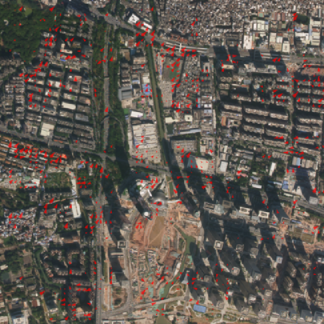
4. Matching points
For each window, that part of the image is compared with the corresponding part of the base map. The algorithm in charge of finding the feature matches is LoFTR1, whose parameters have been optimised for our data by experiments on controlled datasets. The result of this step is a set of points on the image, each with its planimetric distance vector (x, y) to its position on the basemap and a confidence value.
5. Filtering
-
5.1 Confidence: Those points with a confidence value below a threshold value are discarded.
-
5.2 Water: By means of the LULC map, those points on the image that represent water are discarded. In some cases, points on terrain with little or no distinguishable features such as forests can also be discarded. Normally, these points are already filtered out in step 5.1, but this adds an extra security step.
-
5.3 Cloud: By means of the cloud mask associated to the image, those points on the image that represent thick clouds are discarded. Normally, these points are already filtered out in step 5.1, but this adds an extra security step.
-
5.4 Local Outliers factor (LoF) filtering: This and the two following filters aim at detecting and discarding points whose shifts are outliers with respect to the full set of them. This is in order not to consider points where the matching algorithm has made an error with high probability. In particular, we first apply the Local Outlier Factor algorithm, that wants to identify local outliers by measuring the local density deviation of a data point relative to its neighbors.
-
5.5 Global RANSAC: The next outlier filtering step is applying RANSAC to the full set of points. This allows us to detect cases where the previous filter did not succeed and there is a high discrepancy between points coming from applying the LoFTR algorithm to independent windows of the image.
-
5.6 ce90 and RMSE discrepancy: Assuming a tile moves with respect to the basemap in a sort of rigid way, we finally look for points whose shifts are two standard deviations away from the mean of either the x or y shifts distributions.
6. Aggregation and validation
The obtained results for each window are aggregated. KPIs based on the shifts found are calculated as discussed here. Finally, the validity of the result is checked: there must be a minimum number of matches found (see here) and the value of the statistics must be below certain threshold values. This last check is done to rule out complex scenarios where the result is not reliable despite the previous filtering.
Requirements and recommendations
We take requirements and recommendations from the American Society for Photogrammetry and Remote Sensing (ASPRS) standard, which in turn is based on the National Standard for Spatial Data Accuracy standard from the Federal Geographic Data Committee. This section explains the main discrepancies with those requirements and the reason behind them.
Requirements
-
2D positional accuracy shall be tested by comparing the planimetric coordinates of well-defined points. We accept the use of algorithms that compare portions of the image (cell) with the corresponding portion of a basemap to assign to the whole cell a single distance vector. This vector does not refer to a point (pixel) strictly speaking, but reflects an average behaviour of all points (pixels) within the considered cell. It should be noted that when the window does not have any well-defined point, these algorithms are often unable to estimate the distance vector.
-
A minimum of 20 check points shall be tested. We have selected our own threshold in that regard. We found that 30 matching points provided stability and more reliable results.
If 30 or less distance vectors are available, the 2D positional accuracy estimate for that image will be invalidated.
-
For a dataset covering a rectangular area that is believed to have uniform positional accuracy, check points may be distributed so that points are spaced at intervals of at least 10 percent of the diagonal distance across the dataset and at least 20 percent of the points are located in each quadrant of the dataset. We record these requirements but do not use them to rule out an estimate of 2D positional accuracy.
Recommendations
- The accuracy of the control data should be at least three times the accuracy of the analyzed data.
In production we use ESRI as a base map, whose accuracy is variable and unknown.
-
Jiaming Sun et al. LoFTR: Detector-Free Local Feature Matching with Transformers [https://arxiv.org/pdf/2104.00680]. ↩